Notes and resources on basic Machine Learning concepts + ways to try it out.
Overview
Machine learning (ML) lets computers learn from data on their own without requiring software developers to write out all the logic by hand. Given enough data, the machine can learn useful patterns in the data, which turns out to be quite powerful.
The earliest ML algorithms go back to the 1960’s but machine learning started being commonly used in the early 2000’s. In 2012, “deep learning” involving large neural networks became practical and their usage and capabilities has grown exponentially since then.
Basic Machine Learning
It’s best to start with a simple example - let’s say you have a list of heights and weights of people and you want to predict the weight of person in general, given their height.
Height and weight are somewhat correlated, so we can come up with a function to estimate the a person’s weight given their height. Rather than doing this manually, we can put the data into Google Sheets and have it find the formula for the line of best fit.
Try it Yourself
Make a copy of this sheet of heights and weights (Data comes from here.)
Select both columns and click “explore”
Find the scatterplot and drag it into your sheet
To get the line of best fit, double-click the chart and click the “Series” dropdown
Select “Trendline”
This is an extremely simple dataset with only one “feature” to make predictions from (the height) and one predicted value (the weight). Real-world machine learning models can have thousands or millions of features, but the same basic concepts apply to them. Once the best line of fit is found, it can be used to predict future values when only the features are known.
Gradient Descent
The above line of best fit is a linear regression - a simple form of machine learning. How does the computer find the line of best fit?
There are many different algorithms it can use, but a common one throughout machine learning is called Gradient Descent. This algorithm “tries out” a function and then iteratively improves it to minimize the difference between the function’s predictions and the actual data.
More specifically, Gradient Descent guesses a function and then calculates a separate “loss function” which gives a precise measure of the function’s accuracy (generally a simple function such as the “mean squared error”). It can then tweak the actual function’s parameters in the correct direction so that the loss function is minimized. This is like a person descending a mountain:
Imagine you are on the top of a very tall mountain, and your goal is to reach the base of the mountain (which symbolizes the lowest point or minimum value). However, it's really foggy, so you can't see your path to the bottom. What can you do?
You can look at your immediate surroundings, determine which way has the steepest slope downward, and take a step in that direction. You continue this process, always choosing the direction with the steepest downhill slope to take your next step.
This process essentially describes gradient descent:
The mountain represents a cost or loss function, which is a way of quantifying how well the model is performing: the higher up the mountain you are, the worse the model is performing, and vice versa.
The process of determining the steepest slope is equivalent to calculating the gradient (a fancy term for the direction of the steepest slope) of the cost function.
Finally, taking a step in the direction of steepest descent corresponds to updating the model's parameters in a way that makes the model perform better.
Through this iterative process, the model continues to improve its performance, moving closer to the lowest point of the cost function, or in other words, finding the optimal parameters that give the best possible performance.
See also gradient descent for a poetic explanation.
Classification & Logistic Regression
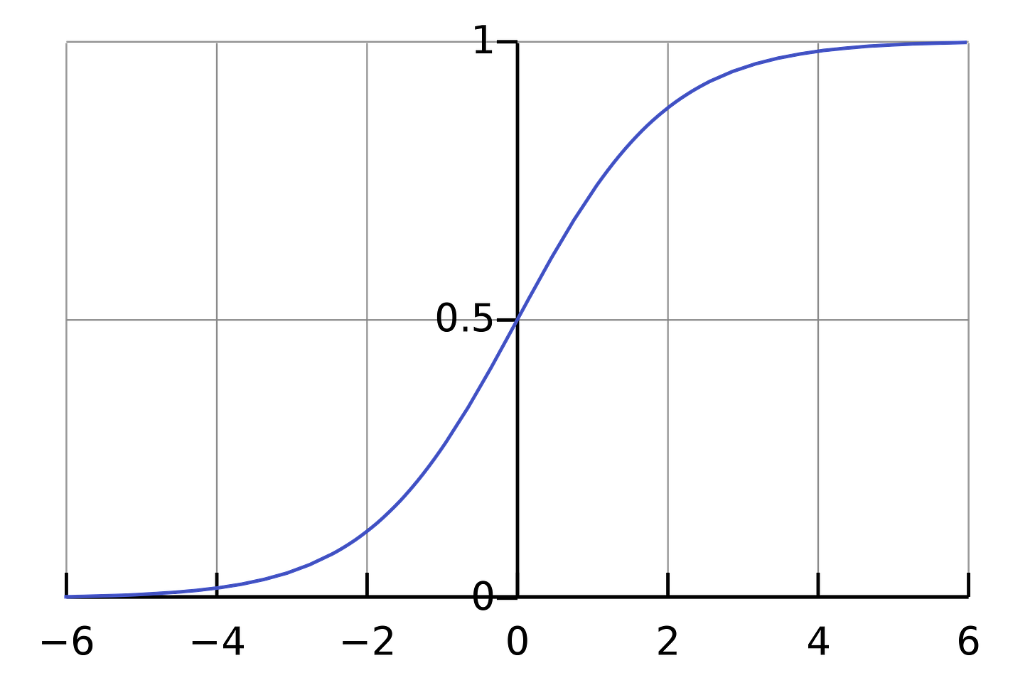
In the above example, we were able to predict a numerical value for a given input. However machine learning is often used for classification to identify whether inputs belong to category or not. For example, it might be used to predict whether email is spam, whether a person will default on their loan, or to identify whether a picture is a cat. In these cases, regular linear regression won’t work as-is, so an additional function is needed to map a numerical output to a classification. Logistic Regression uses a simple “logistic function” to map a linear function into an output value between 0 and 1, which represents the likelihood of input belonging to a class, such as an email being spam.
Neural Networks
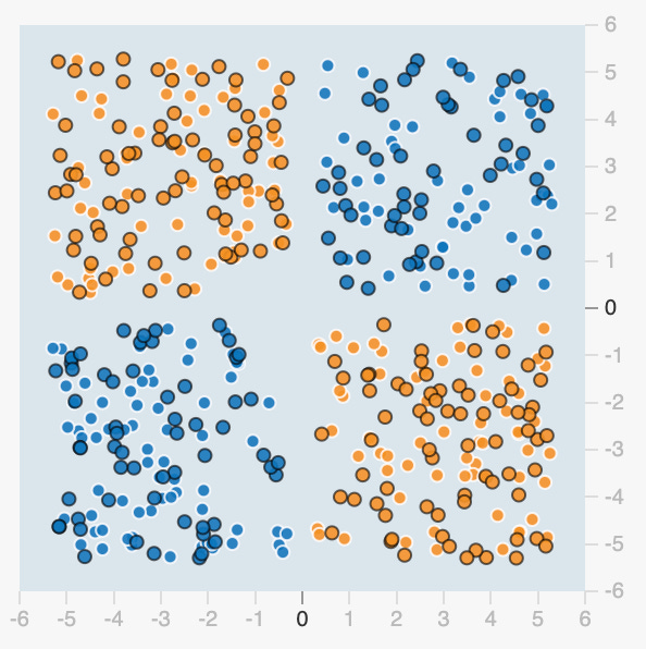
Linear regressions are useful in many cases, but what if a simple linear function can’t accurately model the data? Real-world regression examples often involve complexities that can only be modeled with polynomial, exponential or logarithmic functions. Real-world classification examples often involve complex boundaries that cannot be categorized with a simple linear function. For example, there’s no way to find a linear function that can correctly separate the orange and blue dots in this picture:
A more sophisticated approach is needed, and this is where “artificial neural networks” enter the picture. Neural networks were loosely inspired by the brain and are able to find very complex patterns if given enough data. Here’s how a neural networks works:
It takes in input as numerical values. For example, for image recognition numbers are used to represent the pixels of a picture.
The numbers get sent to “neurons” where each numerical value is multiplied by a numerical weight and and summed together and sent on to the next neurons. In deep learning, multiple layers of neurons are used to help find more complex functions with many variables and nuances.
This network of numbers can help find functions with many variables, but it still can’t find non-linear functions, since each layer in the network just represents a linear function and there’s no way to get a non-linear function by combining multiple linear functions. In order to find non-linear functions, the neurons also use an “activation function” before outputting anything to the next neuron. A common activation function is simply for each node to output 0 for any negative values. This allows the neural network to discover much more complex functions than would otherwise be possible.
The final node in the graph outputs a specific value as the solution to the given input. For example, if the neural network has been trained to recognize cat photos, the final value will be the probability that a the given input represents a cat.
Interacting with a neural network
Real-world neural networks are generally extremely complex and it’s often impossible for humans to understand what’s going on inside them. To see how a neural network works, try out Google’s TensorFlow Playground with simple examples that can be visualized. All the examples involve sample data of orange and blue dots on a 2D grid. Can you figure out the right weights for a neural network so it can predict whether dots should be orange or blue based on their coordinates?
Set the values of your own network
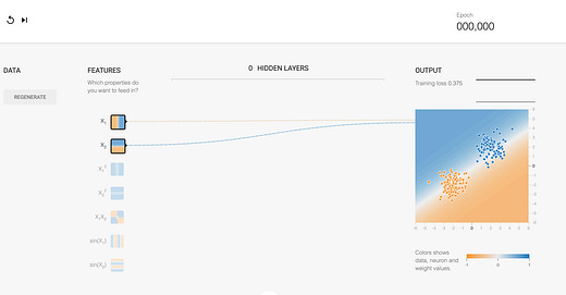
First try it yourself in this simple example with no hidden layers. Click on the lines to set the weights so that the dots are correctly “predicted” by the end.
Note that the X1 input represents the X-coordinate and the X2 input represents the Y-coordinate. After setting weights that work, click refresh and then step forward on top to watch the neural network learn the correct weights on its own.
Neural network with an activation function
Next, try this example with a non-linear distribution. Instead of setting the weights yourself, see if the neural network can learn it by clicking play on top. Try adding a hidden layer so the neural network can learn more complex patterns, and add some neurons to the layer.
The neural network won’t be able to learn the non-linear function here however since everything it’s calculating is still linear.
You have two options to solve this:
a) Add in additional inputs such as the product of the two inputs.
b) Change the activation function so that it’s not linear, e.g. select the ReLU function (which returns 0 for all negative values).
Training & Test Data
This example includes many different settings and knobs, but we’ll focus on one specifically - the test data. When a neural network is training, there’s a risk that it will overfit the data in a way that doesn’t reflect the “reality”. One solution to help address this is to divide the data into “training data” and “test data”. The neural network only uses the training data to determine the weights, but we evaluate how effective it is by running separate test data on it.
Try adding a hidden layer or two and some neurons and then train the neural network so both the training loss and test loss are very low!
To get an intuition for how neural networks work, examine what happens inside the graph as you step through the training process. Observe how sub-patterns emerge that contribute to the final result.
Complex example
Finally, try the most complex example, with all the settings exposed. Can you train a neural network to handle this data correctly? You will again need to add more layers (and maybe more feature inputs) so the neural network can figure it out. After running the neural network, look at the patterns that emerge internally as each node calculates its own “sub-patterns” that contribute to the final solution.
(See bottom of post for possible approaches, and see Google’s machine learning course for more info.)
Backpropogation
How do neural networks figure out what weights to use?
It starts with a guess and does a “forward pass” by passing in the numbers through the network to calculate the results, and then measures the loss function to see how close it was.
It then does backpropogation and goes backwards through the network and nudges the weights to reduce the loss. This process is similar to gradient descent for a linear regression, but it performs it over the weights of the whole neural network.
This is like a company that rapidly manufactures 3D-printed toys with the goal of maximizing their profit.
The work to produce each 3D-printed toy is spit across multiple teams:
The first team analyzes the “raw data” about e.g people’s preferences, the general toy market and the cost of materials. They pass this analysis to the next team - the designers.
The designers sketch out initial concepts for the next batch of toys and pass it to the engineers.
The engineers work out the specific details of how the toys will be printed and what materials to use and pass the plan to the executives.
The executives can make final tweaks before sending the toys to be produced and sold.
Once the toys are sent to market, data is gathered about how well they sels and how profitable it is. Imagine that the toys sell more poorly than expected. The executives learn from these results and send information back to the engineers. The engineers take these results into account and tweak slightly how they think about the finer details of printing and material usage and send the results back to the designers. The designers take this all into account and tweak their design process accordingly. They send the data back to the data processing team, which makes adjustments to how they analyze data. The organization overall is now able to produce better-selling toys going forward.
While this analogy isn’t perfect (humans organizations rarely learn as directly as neural networks!), it helps demonstrate the idea of propagating learning through a network. Each layer of the organization is like a layer in a neural network and they’re all able to learn from a given result. In real neural networks, there may be millions or billions of examples to learn from and they allow tweaking the overall network in a better direction.
It’s surprising how feedback at the end of the process is able to be propagated so effectively through the network. However gradient descent is a very powerful process when given enough data (and computation power) since for each iteration it’s able to tweak all the weights in the right direction. When it does this enough times it eventually reaches a minimum level of error for the data it’s analyzed and the path it took, and it can stop at that point. While it’s not guaranteed to reach the optimal solution in every case, neural networks have worked extremely well in practice for a wide range of problems.
More resources to learn machine learning
High-level concepts
Courses
Elements of AI - Basic machine learning concepts
Coursera - AI for Everyone. See also Supervised Machine Learning to go into some of the technical details.
Free Technical Textbooks
If you’re looking to learn the technical and mathematical details:
Neural Networks and Deep Learning - online book
Deep Learning from MIT, contains more math.
The Little Book of Deep Learning - a mobile-optimized PDF
Tools to Try Machine Learning
Here are some tools from Google that let you try out machine learning:
Simple ML for Sheets - A rudimentary add-on for Sheets.
Teachable Machine - a simple no-code tool for training on images, sounds or poses.
TensorFlow in Colab - actually code with Machine Learning
Appendix - possible approaches to the spiral problem
No special inputs, lots of layers - rely on the neural net to learn the right pattern on its own:
More inputs, less layers - do some “feature engineering” of the inputs to help the neural net learn:


